Windowing Examples
The examples in this section demonstrate how to use LEAD, LAG, and other aggregate functions as window functions in an Expression transformation.
Financial Plans Example
You are a banker with information about the financial plans of two of your customers. Each plan has an associated start date.
For each customer, you want to know the expiration date for the current plan based on the activation date of the next plan. The previous plan ends when a new plan starts, so the end date for the previous plan is the start date of the next plan minus one day.
The following table lists the customer codes, the associated plan codes, and the start date of each plan:
CustomerCode | PlanCode | StartDate |
|---|
C1 | 00001 | 2014-10-01 |
C2 | 00002 | 2014-10-01 |
C2 | 00002 | 2014-11-01 |
C1 | 00004 | 2014-10-25 |
C1 | 00001 | 2014-09-01 |
C1 | 00003 | 2014-10-10 |
|
- Define partition and order keys
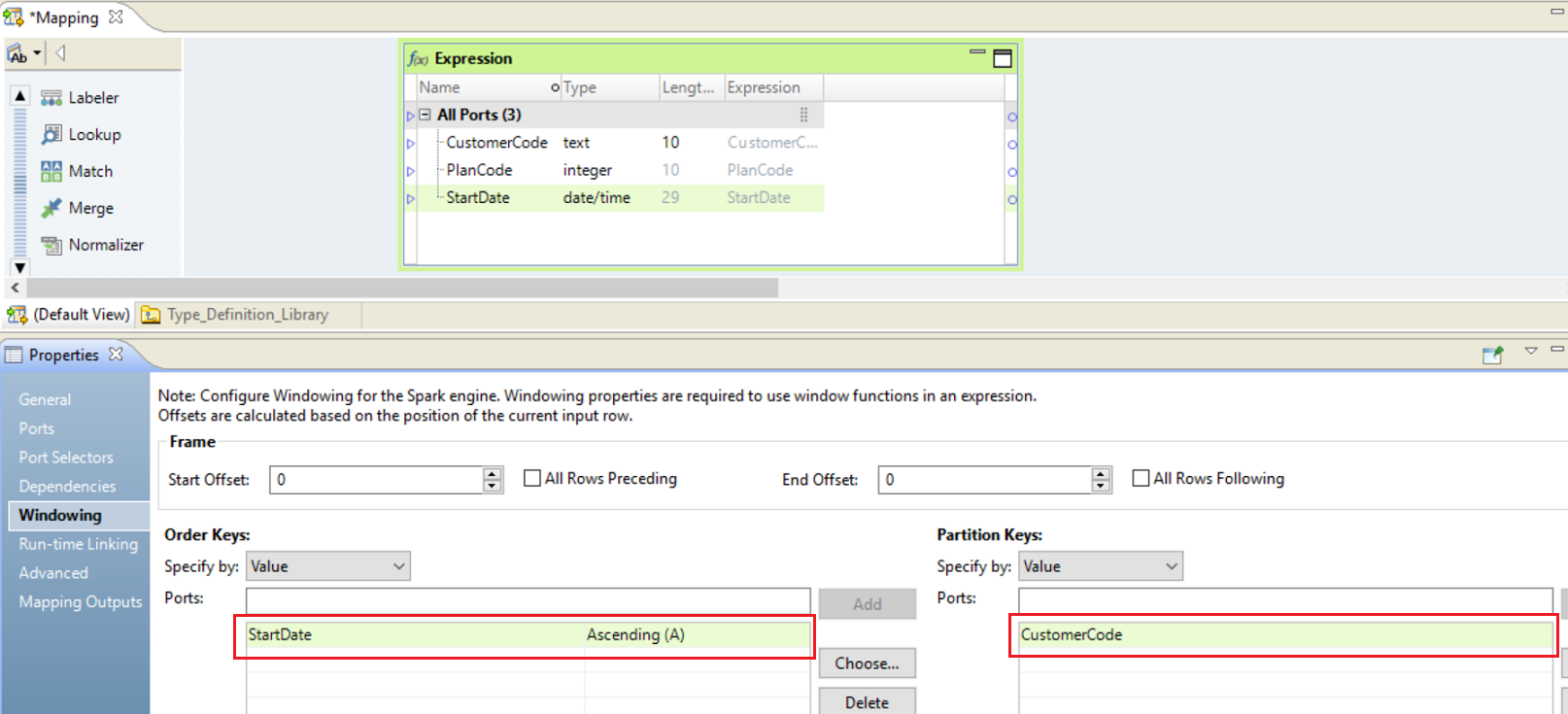
- You partition the data by customer code and order the data by ascending start date.
Property | Description |
|---|
Order key | StartDate Ascending. Arranges the data chronologically by ascending start date. |
Partition key | CustomerCode. Groups the rows according to customer code so that calculations are based on individual customers. |
Frame | Not specified. Window functions access rows based on the offset argument and ignore the frame specification. |
The following table lists the data grouped by customer code and ordered by start date:
CustomerCode | PlanCode | StartDate |
|---|
C1 | 00001 | 2014-09-01 |
C1 | 00002 | 2014-10-01 |
C1 | 00003 | 2014-10-10 |
C1 | 00004 | 2014-10-25 |
C2 | 00001 | 2014-10-01 |
C2 | 00002 | 2014-11-01 |
|
- The start dates for each customer are arranged in ascending order so that the dates are chronological.
- Define a window function
- You define a LEAD function to access the subsequent row for every input.
- You define the following function on the Ports tab of the Expression transformation:
LEAD ( StartDate, 1, '01-Jan-2100' )
Where:
- - StartDate indicates the target column that the function operates on.
- - 1 is the offset. This value accesses the next immediate row.
- - 01-Jan-2100 is the default value. The expression returns "01-Jan-2100" if the returned value is outside the bounds of the partition.
- Define an ADD_TO_DATE function
- You use an ADD_TO_DATE function to subtract one day from the date you accessed.
- You define the following expression on the Ports tab of the Expression transformation:
ADD_TO_DATE ( LEAD ( StartDate, 1, '01-Jan-2100' ), 'DD', -1, )
By subtracting one day from the start date of the next plan, you find the end date of the current plan.
The following table lists the end dates of each plan:
CustomerCode | PlanCode | StartDate | EndDate |
|---|
C1 | 00001 | 2014-09-01 | 2014-09-30 |
C1 | 00002 | 2014-10-01 | 2014-10-09 |
C1 | 00003 | 2014-10-10 | 2014-10-24 |
C1 | 00004 | 2014-10-25 | 2099-12-31* |
C2 | 00001 | 2014-10-01 | 2014-10-31 |
C2 | 00002 | 2014-11-01 | 2099-12-31* |
|
*The LEAD function returned the default value because these plans have not yet ended. The rows were outside the partition, so the ADD_TO_DATE function subtracted one day from 01-Jan-2100, returning 2099-12-31.
GPS Pings Example
Your organization receives GPS pings from vehicles that include trip and event IDs and a time stamp. You want to calculate the time difference between each ping and flag the row as skipped if the time difference with the previous row is less than 60 seconds.
You order the events chronologically and partition the events by trip. You define a window function that accesses the event time from the previous row, and you use an ADD_TO_DATE function to calculate the time difference between the two events.
Windowing Properties
Property | Description |
|---|
Order key | _event_id Ascending. Arranges the data chronologically by ascending event ID. |
Partition key | trip_id. Groups the rows according to trip ID so calculations are based on events from the same trip. |
Frame | Not specified. Window functions access rows based on the offset argument and ignore the frame specification. |
Window Function
You define the following LAG function to get the event time from the previous row:
LAG ( _event_time, 1, NULL )
Where:
- •_event_time is the column name whose value from the previous row is to be returned.
- •1 is the offset. This value represents the row immediately before the current row.
- •NULL is the default value. The function returns NULL if the return value is outside the bounds of the partition.
You define the following DATE_DIFF function to calculate the length of time between the two dates:
DATE_DIFF ( _event_time, LAG ( _event_time, 1, NULL ), 'ss' )
You flag the row as skipped if the DATE_DIFF is less than 60 seconds, or if the _event_time is NULL:
IIF ( DATE_DIFF < 60 or ISNULL ( _event_time ), 'Skip', 'Valid' )
Output
The transformation produces the following outputs:
Trip ID | Event ID | Event Time | Time Difference | Flag |
|---|
101 | 1 | 2017-05-03 12:00:00 | NULL* | Skip |
101 | 2 | 2017-05-03 12:00:34 | 34 | Skip |
101 | 3 | 2017-05-03 12:02:00 | 86 | Valid |
101 | 4 | 2017-05-03 12:02:23 | 23 | Skip |
102 | 1 | 2017-05-03 12:00:00 | NULL* | Skip |
102 | 2 | 2017-05-03 12:01:56 | 116 | Valid |
102 | 3 | 2017-05-03 12:02:00 | 4 | Skip |
102 | 4 | 2017-05-03 13:00:00 | 3480 | Valid |
103 | 1 | 2017-05-03 12:00:00 | NULL* | Skip |
103 | 2 | 2017-05-03 12:00:12 | 12 | Skip |
103 | 3 | 2017-05-03 12:01:12 | 60 | Valid |
|
*The rows preceding these rows are outside the bounds of the partition, so the transformation produced NULL values.
Aggregate Function as Window Function Example
You work for a human resources group and you want to compare each of your employees' salaries with the average salary in his or her department:
The following table lists the department names, the employee identification number, and the employee's salary:
Department | Employee | Salary |
|---|
Development | 11 | 5200 |
Development | 7 | 4200 |
Development | 9 | 4500 |
Development | 8 | 6000 |
Development | 10 | 5200 |
Personnel | 5 | 3500 |
Personnel | 2 | 3900 |
Sales | 3 | 4800 |
Sales | 1 | 5000 |
Sales | 4 | 4800 |
|
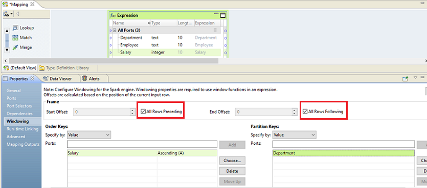
You set an unbounded frame to include all employees in the calculation, and you define an aggregate function to calculate the difference between each employee's salary and the average salary in the department.
Windowing Properties
Property | Description |
|---|
Order key | Salary Ascending. Arranges the data by increasing salary. |
Partition key | Department. Groups the rows according to department. |
Start offset | All Rows Preceding |
End offset | All Rows Following |
With an unbounded frame, the aggregate function includes all partition rows in the calculation.
For example, suppose the current row is the third row. The third row is in the "Development" partition, so the frame includes the third row in addition to all rows before and after the third row in the "Development" partition.
Window Function
An aggregate function acts as a window function when you configure the transformation for windowing.
You define the following aggregate function to calculate the difference between each employee's salary and the average salary in his or her department:
Salary - AVG ( Salary ) = Salary_Diff
Output
The transformation produces the following salary differences:
Department | Employee | Salary | Salary_Diff |
|---|
Development | 11 | 5200 | -820 |
Development | 7 | 4200 | -520 |
Development | 9 | 4500 | 180 |
Development | 8 | 6000 | 180 |
Development | 10 | 5200 | 980 |
Personnel | 5 | 3500 | 200 |
Personnel | 2 | 3900 | 200 |
Sales | 3 | 4800 | -66 |
Sales | 1 | 5000 | -66 |
Sales | 4 | 4800 | 134 |
|
You can identify which employees are making less or more than the average salary for his or her department. Based on this information, you can add other transformations to learn more about your data. For example, you might add a Rank transformation to produce a numerical rank for each employee within his or her department.


